Technology

matlablegend com: MATLAB Legend Guide for Clearer Data Plots!

matlablegend com: A Complete MATLAB Legend Guide With Examples

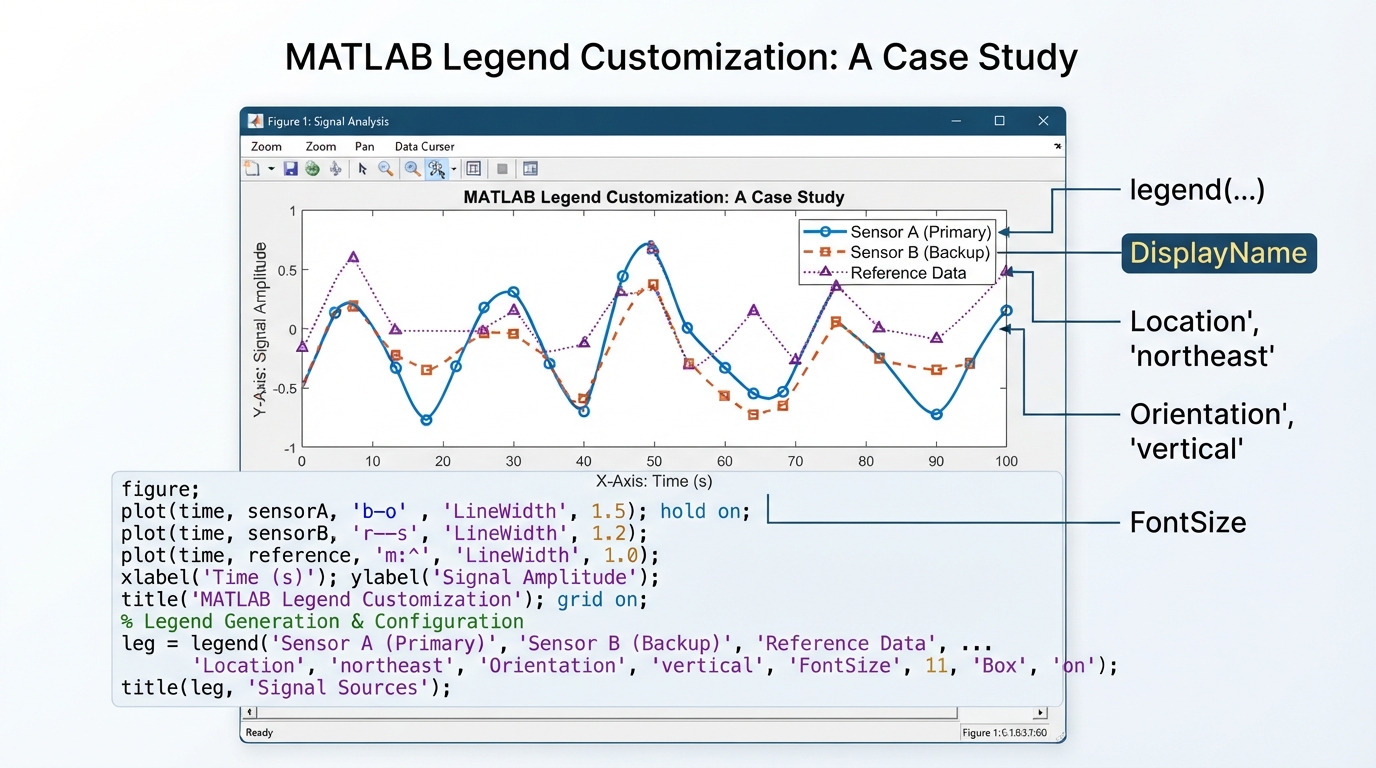
If you searched for matlablegend com because you want a practical explanation of MATLAB legends, the important thing to understand is that the topic is really about making plotted data easier to identify. A MATLAB legend connects visual elements such as lines, markers, bars, or other plotted objects with meaningful labels, so a reader can understand what each series represents without guessing. MATLAB provides the legend function for this purpose, along with properties such as DisplayName, Location, Orientation, NumColumns, and AutoUpdate for more control.

A good legend sounds like a small detail, but it can make the difference between a graph that is immediately understandable and one that forces the reader to inspect every line manually. This guide explains how MATLAB legends work, how to create them, how to position and customize them, how to use DisplayName, how to control which objects appear, and how to troubleshoot the problems that commonly occur.

What Is a Legend in MATLAB?

A legend is a visual key attached to a chart or axes. It associates labels with plotted data series.

Suppose you plot temperature measurements for three cities on the same graph. Without a legend, the reader may see three lines but have no reliable way to know which line belongs to which city.

A legend solves that problem by displaying labels such as:

New York

London

Tokyo

alongside visual samples representing the corresponding plotted series.

In practical terms, a MATLAB legend answers a simple question:

“What does each object in this graph represent?”

This becomes particularly important when several curves share the same axes. The more data series a chart contains, the more valuable clear labeling becomes.

MATLAB’s legend function is specifically designed to add this descriptive information to plots. The official MATLAB documentation also places legends alongside titles, axis labels, annotations, and other tools used to make graphics easier to interpret.

Why MATLAB Legends Matter

A graph can contain accurate data and still be difficult to understand.

Imagine a research plot containing six curves. Each curve may represent a different experiment, algorithm, parameter value, or physical condition. If the lines are not labeled, the reader has to infer their meaning from the surrounding text.

That creates unnecessary cognitive work.

A well-designed legend provides context directly inside the figure.

This is especially useful in:

Research papers

Engineering reports

Laboratory results

Scientific simulations

Machine learning experiments

Signal processing

Financial charts

Data analysis dashboards

Academic assignments

Technical presentations

The goal is not simply to add a box to a graph. The goal is to make the relationship between the visual data and its meaning obvious.

The Basic MATLAB Legend Syntax

The simplest form is:

legend(‘Label 1′,’Label 2’)

For example:

x = 0:0.1:10;

y1 = sin(x);

y2 = cos(x);

plot(x,y1)

hold on

plot(x,y2)

hold off

legend(‘Sine’,’Cosine’)

The first label is associated with the first plotted series, while the second label is associated with the second series.

This order matters.

If you plot one line and then another line, the labels supplied to legend normally correspond to those plotted objects in their relevant order.

This basic behavior is also demonstrated in MATLAB educational material, where multiple functions are plotted and then identified through the legend command.

A Simple Example With Two Curves

Here is a complete example that is easy to test:

x = linspace(0,2*pi,200);

y1 = sin(x);

y2 = cos(x);

plot(x,y1)

hold on

plot(x,y2)

hold off

legend(‘sin(x)’,’cos(x)’)

xlabel(‘x’)

ylabel(‘Value’)

title(‘Sine and Cosine Functions’)

The resulting chart contains two curves.

The legend tells the reader which curve represents sin(x) and which represents cos(x).

This is one of the most common uses of MATLAB legends and is a useful starting point before moving into more advanced techniques.

Using DisplayName Instead of Manually Writing Labels

For larger scripts, repeatedly maintaining the labels inside a separate legend() command can become inconvenient.

MATLAB provides another approach through the DisplayName property.

You can assign a descriptive name when creating the plotted object:

x = linspace(0,5);

y1 = sin(x);

y2 = cos(x);

plot(x,y1,’DisplayName’,’Sine’)

hold on

plot(x,y2,’DisplayName’,’Cosine’)

hold off

legend

Here, each plotted object carries its own label.

This approach becomes particularly useful when a script grows over time. If another data series is added, its label can be defined directly with the object.

For example:

plot(x,tan(x),’DisplayName’,’Tangent’)

The DisplayName property is recognized by MATLAB’s legend system. When no descriptive name is provided, MATLAB can fall back to labels such as dataN, which are usually less useful to readers.

Why DisplayName Is Useful in Larger MATLAB Projects

Consider a script that creates ten different plots.

With a traditional approach, you might need to remember the order of all ten plotting commands and then provide ten labels later.

That increases the chance of a mismatch.

With DisplayName, the description stays attached to the corresponding graphical object.

For example:

plot(x,y1,’DisplayName’,’Experimental Data’)

hold on

plot(x,y2,’DisplayName’,’Model Prediction’)

plot(x,y3,’DisplayName’,’Reference Curve’)

hold off

legend

The code becomes easier to maintain because the meaning of each series is visible at the point where it is created.

This is one reason DisplayName is particularly helpful in scripts used for research, engineering, and automated visualization.

MATLAB Legend Location

A legend can occupy different positions around the axes.

For example:

legend(‘Sine’,’Cosine’,’Location’,’northwest’)

places the legend in the upper-left area of the axes.

Common location values include:

Location	Meaning
north	Top inside the axes
south	Bottom inside the axes
east	Right side inside the axes
west	Left side inside the axes
northeast	Upper-right inside the axes
northwest	Upper-left inside the axes
southeast	Lower-right inside the axes
southwest	Lower-left inside the axes
northoutside	Above the axes
southoutside	Below the axes
eastoutside	Right of the axes
westoutside	Left of the axes
best	Position selected to reduce overlap
bestoutside	Outside position selected for reduced conflict

The current MATLAB documentation includes additional location choices for modern graphics layouts, including outside-corner positions and layout for tiled charts.

When Should You Use Location Best?

If you are not sure where the legend should go, try:

legend(‘Location’,’best’)

MATLAB attempts to place the legend where it interferes least with the plotted data.

This is convenient for exploratory work.

However, best is not always the best choice for a final publication figure. If the graph changes later, the automatically selected position can also change.

For a report, paper, or presentation, it is often better to inspect the final figure and choose a deliberate position.

Putting the Legend Outside the Plot

Sometimes the data occupies most of the plotting area.

In that situation, putting the legend inside the axes can cover important information.

You can move it outside:

legend(‘Sine’,’Cosine’,’Location’,’eastoutside’)

This places the legend on the right side.

Another useful option is:

legend(‘Sine’,’Cosine’,’Location’,’northoutside’)

This places the legend above the axes.

Outside placement can be especially useful for charts containing dense curves, annotations, or large data markers.

Changing Legend Orientation

By default, legend entries are generally arranged vertically.

You can request a horizontal arrangement:

legend({‘Sine’,’Cosine’}, …

‘Orientation’,’horizontal’)

This can work well when there are only a few labels.

For example, a report figure with three short labels may look cleaner with all three entries arranged across the top rather than stacked vertically.

MATLAB supports both vertical and horizontal orientations.

Using a Legend Object

MATLAB can return the legend as an object.

For example:

lgd = legend(‘Sine’,’Cosine’);

Now lgd represents the Legend object.

You can use it to modify properties after creation.

For example:

lgd = legend(‘Sine’,’Cosine’);

lgd.FontSize = 14;

You can also add a title:

lgd.Title.String = ‘Functions’;

This approach is useful when several legend properties need to be changed.

The current MATLAB examples also demonstrate modifying the legend through an object and using properties such as FontSize and Title.

Changing the Font Size

A readable legend should match the visual hierarchy of the rest of the chart.

You can change the font size with:

lgd = legend(‘Sine’,’Cosine’);

lgd.FontSize = 12;

If the graph is intended for a presentation, a slightly larger font may be appropriate.

For a dense research figure, however, increasing the font too much can make the legend occupy excessive space.

The right choice depends on the figure’s final display size.

Adding a Legend Title

A legend can also have a title.

For example:

lgd = legend(‘Training’,’Testing’);

lgd.Title.String = ‘Dataset’;

The result communicates that the legend entries belong to a particular category.

This can be helpful when labels alone are ambiguous.

For example, instead of:

you might have:

Model

A legend title should be used when it adds information, not simply because the feature exists.

Creating a Multi-Column Legend

A long vertical legend can consume considerable space.

MATLAB supports multiple columns through the NumColumns property.

For example:

x = linspace(0,10);

plot(x,sin(x),’DisplayName’,’sin(x)’)

hold on

plot(x,sin(0.9*x),’DisplayName’,’sin(0.9x)’)

plot(x,sin(0.8*x),’DisplayName’,’sin(0.8x)’)

plot(x,sin(0.7*x),’DisplayName’,’sin(0.7x)’)

plot(x,sin(0.6*x),’DisplayName’,’sin(0.6x)’)

plot(x,sin(0.5*x),’DisplayName’,’sin(0.5x)’)

hold off

lgd = legend;

lgd.NumColumns = 2;

This divides the legend into two columns.

It is particularly useful when a chart contains many series.

The recent MATLAB legend examples also use NumColumns to organize six plotted curves into a more compact legend.

Showing Only Selected Data Series

Not every object in a graph needs to appear in the legend.

Suppose you have two bar charts and one scatter plot, but you only want the two bar charts represented.

You can keep handles to the desired objects:

x = 1:5;

y1 = [2 4 6 4 2];

b1 = bar(x,y1);

hold on

y2 = [1 3 5 3 1];

b2 = bar(x,y2);

y3 = [2 4 6 4 2];

s = scatter(x,y3,’filled’);

hold off

legend([b1 b2],’Bar Chart 1′,’Bar Chart 2′)

The first argument specifies the graphics objects that should be represented.

This gives you much more control than simply supplying labels in sequence.

MATLAB’s current documentation and recent examples support passing specific graphics objects to legend for selective inclusion.

MATLAB Legend With a Bar Chart

Legends are not limited to line graphs.

For example:

categories = 1:4;

sales = [15 22 18 30];

bar(categories,sales)

legend(‘Sales’)

xlabel(‘Quarter’)

ylabel(‘Units’)

title(‘Quarterly Sales’)

The legend identifies the bar series.

When multiple bar groups are plotted, separate labels can be provided:

x = 1:4;

online = [20 25 30 35];

store = [15 18 24 28];

bar(x,[online’ store’])

legend(‘Online’,’Store’)

Now the legend explains the two data series.

MATLAB Legend With Scatter Plots

Scatter plots can also use legends.

For example:

x1 = [1 2 3 4 5];

y1 = [2 3 5 4 6];

x2 = [1 2 3 4 5];

y2 = [6 5 4 3 2];

scatter(x1,y1,’filled’,’DisplayName’,’Group A’)

hold on

scatter(x2,y2,’filled’,’DisplayName’,’Group B’)

hold off

legend

Using DisplayName here avoids having to manually maintain the labels separately.

The MATLAB graphics system supports DisplayName for scatter objects as a legend label.

How Legend Auto-Update Works

One useful MATLAB behavior is that legends can update when plotted objects are added or removed.

For example:

x = linspace(0,5);

plot(x,sin(x),’DisplayName’,’Sine’)

hold on

plot(x,cos(x),’DisplayName’,’Cosine’)

legend

If another object is added with an appropriate DisplayName, MATLAB can incorporate it into the legend.

For example:

plot(x,sin(2*x),’DisplayName’,’Sine 2x’)

The AutoUpdate property controls whether the legend responds to changes in the axes contents. MATLAB documentation notes that automatic updating can be disabled when you want the legend to remain fixed.

To turn it off:

lgd = legend;

lgd.AutoUpdate = ‘off’;

This can be useful when a script adds helper objects that you do not want appearing in the legend.

How to Stop Unwanted Objects From Appearing

A common problem occurs when a graph contains objects that are useful for the visualization but should not be described in the legend.

For example, you might add a reference line.

If you do not want that object represented, you can control legend inclusion through graphics object properties or by explicitly specifying which objects belong in the legend.

One approach is to create handles for the objects you actually want:

p1 = plot(x,y1);

hold on

p2 = plot(x,y2);

yline(5);

hold off

legend([p1 p2],’Experiment’,’Model’)

This is often easier to understand than trying to remove unwanted entries afterward.

How to Remove a MATLAB Legend

If you no longer need the legend, use:

legend(‘off’)

For example:

x = 0:0.1:10;

plot(x,sin(x))

legend(‘Sine’)

legend(‘off’)

The legend is removed from the current axes.

This is useful in scripts where the same figure is reused for different outputs.

The legend(‘off’) behavior is part of MATLAB’s standard legend functionality and is also documented in educational references.

What Happens If You Do Not Provide DisplayName?

Suppose you write:

plot(x,y1)

hold on

plot(x,y2)

legend

MATLAB still needs to identify the objects.

If no DisplayName values have been supplied, generic labels may be assigned.

Depending on the graphics objects and MATLAB version, these can take forms such as data1, data2, and similar automatically generated names.

These labels technically identify separate objects, but they do not tell the reader what the data means.

Compare:

data1

data2

with:

Measured Pressure

Predicted Pressure

The second version is much more informative.

For that reason, meaningful DisplayName values are preferable whenever the chart is intended for someone other than the person who created it.

Common MATLAB Legend Problem: Labels Do Not Match the Lines

One of the most frustrating mistakes is supplying labels in the wrong order.

For example:

plot(x,y1)

plot(x,y2)

plot(x,y3)

legend(‘Third’,’First’,’Second’)

The graph may display a legend, but the descriptions do not represent the intended curves.

The safest solution is to maintain a clear relationship between plotting order and labels.

An even better approach for larger scripts is often:

plot(x,y1,’DisplayName’,’First’)

hold on

plot(x,y2,’DisplayName’,’Second’)

plot(x,y3,’DisplayName’,’Third’)

hold off

legend

Now each label is associated with its own plotted object.

Common MATLAB Legend Problem: Legend Covers the Data

If the legend sits directly over an important curve, change its position.

Try:

legend(‘Location’,’best’)

If that is not suitable, explicitly choose another location:

legend(‘Location’,’northwest’)

or:

legend(‘Location’,’eastoutside’)

The right location depends on where the data is concentrated.

For example, if the upper-right region contains an important peak, placing the legend at northeast may obscure it.

Common MATLAB Legend Problem: Too Many Legend Entries

A chart with fifteen plotted objects does not necessarily need fifteen legend entries.

Some objects may be:

Reference lines

Grid helpers

Confidence boundaries

Annotations

Background elements

Intermediate visualization objects

In such cases, specify the exact objects that should appear:

legend([p1 p2 p3], …

‘Observed’,’Predicted’,’Reference’)

This keeps the figure focused.

A good rule is simple: if a legend entry does not help the reader interpret the graph, consider leaving it out.

Common MATLAB Legend Problem: The Legend Is Too Large

If labels are long, the legend can become wider or taller than the actual plot.

Start by shortening labels.

Instead of:

Experimental measurements collected during the first testing condition

consider:

Experiment 1

If the longer explanation is important, put it in the figure caption or surrounding text.

You can also use multiple columns:

lgd = legend;

lgd.NumColumns = 2;

Or move the legend outside the axes.

How to Make MATLAB Legends More Professional

A technically correct legend is not necessarily a visually effective legend.

For professional figures, think about readability.

Use descriptive but concise labels.

Avoid unnecessary repetition.

Do not cover important data.

Keep the font readable.

Use consistent terminology.

Make sure the legend corresponds exactly to the visual encoding.

If the graph uses line styles, markers, or colors to distinguish series, the legend should make those relationships obvious.

A reader should be able to look at the chart and understand the mapping within seconds.

Legend Versus Axis Labels

A legend and an axis label serve different purposes.

The x-axis label describes what the horizontal dimension represents.

The y-axis label describes what the vertical dimension represents.

The legend identifies multiple data series.

For example:

xlabel(‘Time (s)’)

ylabel(‘Temperature (°C)’)

legend(‘Sensor A’,’Sensor B’)

Here, the axis labels establish the coordinate system while the legend distinguishes the sensors.

A complete visualization may need all three.

Legend Versus Chart Title

The title provides the overall context of the graph.

The legend provides series-specific information.

For example:

title(‘Temperature Measurements’)

xlabel(‘Time (minutes)’)

ylabel(‘Temperature (°C)’)

legend(‘Indoor’,’Outdoor’)

The title tells the reader what the figure is about.

The axes explain the variables.

The legend explains which line belongs to which measurement.

These elements work together rather than replacing one another.

A Practical MATLAB Legend Example

Here is a more realistic example using measured and predicted values:

time = 0:1:10;

measured = [20 22 24 25 27 29 31 32 34 35 37];

predicted = [19 21 23 26 28 30 30 33 35 36 38];

plot(time,measured,’o-‘,’DisplayName’,’Measured’)

hold on

plot(time,predicted,’–‘,’DisplayName’,’Predicted’)

hold off

xlabel(‘Time (hours)’)

ylabel(‘Temperature (°C)’)

title(‘Measured vs Predicted Temperature’)

lgd = legend;

lgd.Location = ‘northwest’;

lgd.FontSize = 11;

This example demonstrates several good practices.

The data series have meaningful names.

The axis labels explain the variables.

The title provides context.

The legend is positioned deliberately.

The visual styles distinguish the two series.

The code is also easy to extend.

A Better Approach for Dynamic Data

When the number of series changes dynamically, DisplayName can make the code more manageable.

For example:

x = linspace(0,10);

for k = 1:3

y = sin(k*x);

plot(x,y,’DisplayName’,sprintf(‘Signal %d’,k))

hold on

end

hold off

legend

The labels are generated automatically.

This approach is particularly useful for scripts that process multiple experiments or datasets.

Instead of manually changing the legend every time the number of series changes, the plotting code generates the labels as part of the loop.

MATLAB Legend and Multiple Axes

When working with multiple axes, it is important to know which axes the legend belongs to.

You can explicitly specify the target axes when needed.

This becomes useful in figures containing several subplots or more complex layouts.

For example, if you have a specific axes handle:

ax = axes;

plot(ax,x,y1,’DisplayName’,’Series A’)

hold(ax,’on’)

plot(ax,x,y2,’DisplayName’,’Series B’)

legend(ax)

This makes the intended target explicit.

It can reduce confusion in larger visualization scripts where several axes exist simultaneously.

Using Legends in Subplots

Suppose a figure contains multiple plots:

subplot(2,1,1)

plot(x,y1,’DisplayName’,’Signal A’)

hold on

plot(x,y2,’DisplayName’,’Signal B’)

legend

subplot(2,1,2)

plot(x,y3,’DisplayName’,’Signal C’)

hold on

plot(x,y4,’DisplayName’,’Signal D’)

legend

Each axes can have its own legend.

This is often preferable when each subplot tells a different story.

If all subplots share the same interpretation, however, a carefully designed common legend may produce a cleaner final figure.

Should Every MATLAB Plot Have a Legend?

No.

A legend is useful when the reader needs help distinguishing multiple plotted series.

If the graph contains only one line and the title or surrounding text already identifies it clearly, a legend may be unnecessary.

For example:

plot(x,y)

title(‘Daily Revenue’)

xlabel(‘Day’)

ylabel(‘Revenue’)

Adding a single legend that simply says Revenue may not provide much additional information.

Good visualization is about clarity, not adding every available feature.

MATLAB Legend Best Practices

A strong legend usually follows a few straightforward principles.

Use meaningful names rather than generic labels.

Keep labels short enough to scan quickly.

Position the legend where it does not hide important data.

Use DisplayName when managing multiple plotted objects.

Use NumColumns when a large number of entries makes the legend unnecessarily tall.

Specify selected graphics objects when only certain data series should appear.

Turn AutoUpdate off when later plotting commands should not modify an established legend.

Review the final figure at the size at which readers will actually see it.

These practices are more important than simply knowing the syntax.

MATLAB Legend Syntax Cheat Sheet

Task	Example
Create a legend	legend(‘A’,’B’)
Use existing DisplayName values	legend
Set location	legend(‘Location’,’northwest’)
Horizontal orientation	legend(‘Orientation’,’horizontal’)
Remove legend	legend(‘off’)
Save legend object	lgd = legend
Change font size	lgd.FontSize = 12
Add legend title	lgd.Title.String = ‘Data’
Multiple columns	lgd.NumColumns = 2
Disable automatic updates	lgd.AutoUpdate = ‘off’
Select specific objects	legend([p1 p2],’A’,’B’)
Set label through plotting command	plot(x,y,’DisplayName’,’Series A’)

This gives you the most commonly needed operations in one place.

Frequently Asked Questions About MATLAB Legend

What does the legend command do in MATLAB?

The legend command creates or controls a legend associated with plotted data. It helps identify which visual element corresponds to each data series.

How do I add a legend to a MATLAB plot?

Plot your data first and then call:

legend(‘Series 1′,’Series 2’)

The labels correspond to the relevant plotted series.

How do I automatically label MATLAB plots?

Use the DisplayName property:

plot(x,y,’DisplayName’,’My Data’)

legend

This lets the legend use the descriptive name attached to the graphics object.

How do I change the MATLAB legend position?

Use the Location property:

legend(‘Location’,’northwest’)

You can also use positions such as south, eastoutside, westoutside, best, and other supported values.

How do I put a MATLAB legend outside the graph?

Use an outside location, such as:

legend(‘Location’,’eastoutside’)

This places the legend outside the plotting area.

How do I make a horizontal MATLAB legend?

Use:

legend(‘Orientation’,’horizontal’)

This arranges legend entries horizontally rather than vertically.

How do I remove a legend in MATLAB?

Use:

legend(‘off’)

This removes the legend from the current axes.

Can MATLAB legends have multiple columns?

Yes. Retrieve the Legend object and set NumColumns:

lgd = legend;

lgd.NumColumns = 2;

This is useful for figures with many series.

Why does MATLAB show data1 and data2 in my legend?

This generally happens when the plotted objects do not have useful DisplayName values. Assign meaningful names through DisplayName or provide labels directly to legend.

Can I show only selected plots in a legend?

Yes. Pass the desired graphics object handles to legend:

legend([p1 p2],’Experiment’,’Prediction’)

This is useful when helper objects should remain out of the legend.

Does MATLAB automatically update legends?

A legend can automatically respond when data series are added or removed. The AutoUpdate property can be used to control this behavior.

Final Takeaway

A MATLAB legend is much more than a decorative box placed beside a graph. It is part of the communication layer of a visualization.

When several curves, bars, markers, or other objects appear on the same axes, the legend gives those visual elements meaning. MATLAB makes the process straightforward with the legend function, while features such as DisplayName, Location, Orientation, NumColumns, object handles, and AutoUpdate provide the control needed for more advanced figures. Also read this Adstotally.com Explained: What It Really Is in 2026

For simple charts, this may be enough:

legend(‘Sine’,’Cosine’)

For larger projects, a more maintainable approach is:

plot(x,y1,’DisplayName’,’Measured’)

hold on

plot(x,y2,’DisplayName’,’Predicted’)

hold off

legend

The biggest lesson is to treat the legend as part of the explanation of your data. Use labels that communicate meaning, position the legend where it does not obstruct the visualization, and avoid adding entries that do not help the reader.

If you are learning MATLAB, mastering these techniques will make your plots easier to understand and your scripts easier to maintain. For official syntax and the latest supported properties, the MathWorks MATLAB legend documentation is the best technical reference.